Random failure is exponential reliability decay

When something decays or grows “exponentially” it means that it changes regularly by a constant factor. An example of exponential growth is the principle in a compound interest bank account which increases at regular intervals by a constant factor^[1]. Assume that you drive your car normally. You replace tires whenever the tread depth falls below the manufacturer’s safety recommendation. ^[2] Intuitively, we would agree that you’re no more likely to have a punctured tire in any one year than in any other.^[3]

In other words the conditional probability of failure (a flat tire) is constant or age independent. We call this failure pattern “random”.^[4]  Assume that the conditional failure probability of a puncture in any year is a constant 25%.  When you drive the car off the dealer’s lot for the first time, at that moment the Reliability R1 is 100%. What is the Reliability R2 at the beginning of the second year?  In the article here we showed the Conditional Probability of Failure to be:

(1)  

Rearranging and substituting

(2)  

The reliability at the beginning of year 3 is:

(3)  

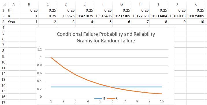
Repeating the calculation in an Excel spreadsheet for each subsequent year reveals the exponentially decaying Reliability curve:

The Reliability graph says that there is a 7.5% chance (row 2 col K) that you will drive for 9 years without a puncture.^[5]

Discrete versus continuous reliability analysis

In the article Random failure and the MTTF we showed that the equation describing the exponential decay of Reliability (random failure) is: . Let us include this equation in our Excel worksheet (in row 27). In rows 20 to 26 we set up the following example: Assuming a sample of 100 cars there will be 75 survivors at the beginning of year two at which time 100 car years will have been logged, 56.25 survivors at the start of year 3 at which time 175 failure free car years will have been logged, and so on. The MTTF = 4 will be calculated (in row 26) as the total number of car years 369.97 divided by the number of failures 92.49 in the period:

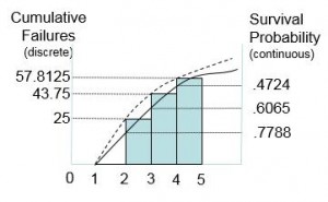
Note that the Reliability as calculated by the equation for random failure (row 27) is different from that calculated in row 2 and suggested by the number of survivors (row 20) at the start of each year. That is because the Reliability equation represents a continuous function while the Survivors were calculated in the worksheet at discreet intervals as if all failures occurred on the last day of each year. They would actually have been spread out over the year.

Histogram of the accumulating failures (from row 21) in each year. The dashed curve represents the discrete calculation. The solid curve drawn through the mid point of each interval predicts the accumulated failures from the continuous Cumulative Failure Probability function (the complement of the Reliability function).

It would be more reasonable to use the middle of the year in the histogram of cumulative failures (from row 21) as representative of the average time of failure in each interval.

Hence the continuous Reliability Curve  of row 27 would show somewhat better survival levels at year start than the discrete calculation (row 2). Accordingly row 27 (col K) shows that your chances of driving for nine years without  a puncture would be closer to 10.5% than to 7.5% as determined from the discrete calculation of row 2. For more information on discrete versus continuous reliability calculation see the articles here and here.

© 2014 – 2016, Murray Wiseman. All rights reserved.

1. ^[1]The factor is 1 plus the interest rate↩
2. ^[2]This is an example of applying a Preventive Maintenance strategy in order to gain the desired constant, low conditional failure probability pattern. If we allow the treads to wear beyond the safety depth then tire failure would become age related meaning that the conditional probability of failure would increase with age  conforming to Nowlan and Heap’s pattern B.↩
3. ^[3]Nevertheless the probability of surviving to an age t decreases with increasing age because, obviously, if you keep driving the car, eventually you will have a flat. This does not contradict the fact (although it seems paradoxical) that the probability of getting a flat in any one year, if you ask the question at the start of the year, remains constant.↩
4. ^[4]The word “random” when used in the reliability sense differs from the often conjured image of throwing dice. In the latter situation it is impossible to predict the result of the next throw. To the reliability engineer, however, “random” means merely that the conditional failure probability in any interval is independent of the item’s age. Therefore, even when an item’s failure behavior is random, observed condition data can be used to predict its failure.↩
5. ^[5]Sometimes engineers might argue that if you replace tires whenever the tread depth reaches the safety limit then the survival curve for a tire will go back up to 100% at that time, so that we no longer have exponential decay. They would be correct if we were dealing with a failure mode subject to wear out. But in this case we are considering only a puncture due to a nail or broken glass on the road. It is going to be exponential decay no matter how often you replace the tires because the probability of getting a puncture is the same in any interval no matter the tire’s age as long as you are above the safety limit. ↩