EXAKT cost sensitivity analysis

Progress seldom proceeds smoothly. It occurs in steps. A new strategy of some kind usually precedes each step. If the strategy is right the individual or organization moves forward and benefits. The wrong strategy, however, will generate decisions that delay or even reverse progress. Often the long term results of a strategy are not obvious. How then can we judge the worth of our strategy or the validity of its assumptions?

In the management of physical assets strategies are called “policies”. And those policies govern day-to-day decisions as to what maintenance actions to perform and when to perform them. Managers and engineers develop or inherit maintenance policies.^[1] In either case they should periodically question the assumptions upon which a current policy is based. Furthermore, they should have a way to test assumptions when considering a new or proposed policy. The Mesh™ LRCM data enabled EXAKT process uses cost sensitivity analysis to examine the validity of a key assumption, namely, the failure penalty relative to the failure mitigating cost associated with a given CBM policy.

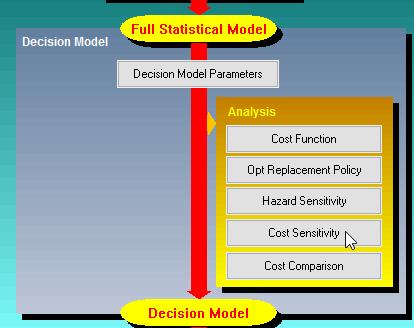
In this article we’ll revisit Exercise 1 in order to conduct a cost sensitivity analysis of a given CBM policy. The questions we should ask are: How will the benefits ascribed to the policy be affected if its assumptions  are inaccurate or if the asset’s operating context has changed? Will the policy still be optimal? Is CBM still justified? Should we exert additional CBM effort? To answer these questions begin by repeating steps 1 to 5 in the article Measuring CBM Effectiveness and then hit the Cost Sensitivity button as shown in the image above.

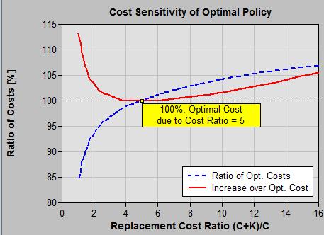
This will display the Cost Sensitivity of Optimal Policy graph as shown in the image below. From the graph you will be able to judge the impact of cost variations on the model’s performance. In other words, for a model you have developed, you can see whether you need to have only a rough estimate of the relative failure and preventive costs, or if you need a more precise one.

Two curves are shown in the Cost Sensitivity of Optimal Policy graph: 1) Ratio of Optimal Costs (blue dashed curve),  and 2) Increase over Optimal Cost (red solid curve). The intersection shows the cost ratio (C+K)/C of 5^[2] used to build the model of Exercise 1.

Define the “Maintenance Cost” MC = preventive  cost C and reactive cost C+K per unit of working age.^[3]

1. Reading the blue dashed curve:
   • The y-axis compares^[4] the  MC of a model operating under a different (C+K)/C ratio with the same model operating under its original (C+K)/C ratio.
   • So in Example 1 if the (C+K)/C ratio were to increase from 5 to 12 the MC would increase to 105% of the optimal cost that was calculated when developing the original model. That is to say, a failure penalty K large enough to increase the (C+K)/C ratio to 12 will increase MC by 5%.
   • And a smaller failure penalty than originally input to the model will decrease MC according to the graph.
2. Reading the Red solid curve:
   • Say you built your current policy assuming a (C+K)/C ratio of 5. But the real (C+K)/C ratio is 12. So the current policy is not optimal.
   • Now say you rebuild the policy with the correct (C+K)/C = 12 so that it is optimal.
   • The solid red line compares the current non-optimal policy’s MC to the MC of the optimal policy re-developed with the (C+K)/C ratio of 12 yielding a MC increase of 2.5%.
   • So in the example of Exercise 1, regardless of the above numbers we can say from the shape of the red solid curve, that our policy remains close to optimal (lowest cost) for (C+K)/C ratios that range from about 4 to about 7. Outside that range we should recalculate and use the new decision policy.

Summarizing, once the optimal decision policy is calculated, we can analyze its sensitivity to changes in the (C+K)/C cost ratio. The Cost Sensitivity function of EXAKT gives us  a detailed analysis of the changes in the cost of the optimal policy due to changes in the  ratio. This analysis is quick and easy^[5]. When carried out periodically by the reliability engineer the Cost Sensitivity analysis may trigger a recalculation and deployment of a new CBM decision policy.

© 2015 – 2016, Murray Wiseman. All rights reserved.

1. ^[1]Maintenance polices, ideally, will have been documented inside an RCM analysis.↩
2. ^[2]C is the recurrent cost of proactive maintenance (renewal) directed at mitigating the consequences of failure. The economic failure consequences are referred to in this article as the “failure penalty” K. Hence K is the cost of a failure over and above the cost C of preventive renewal or repair. ↩
3. ^[3]More precisely, MC is the expected annual cost of maintenance which would be equal to the number of times in a year preventive maintenance will have been carried out multiplied by C plus the number of times failure maintenance will have had to be performed multiplied by C+K↩
4. ^[4]as a ratio of the current cost situation to the optimal cost as calculated in the development of the model↩
5. ^[5]presupposing that a living RCM (LRCM) process is in place so that the EAM database is of analytical quality↩